Exploring Ways to Get Copilot Capacity with Fabric

Maximizing Efficiency and Cost-Effectiveness

In today’s fast-paced digital environment, businesses are constantly seeking ways to streamline operations and enhance productivity. One of the most innovative solutions in the realm of cloud computing is the deployment of copilot capacities with Fabric, a powerful tool that allows companies to leverage artificial intelligence and machine learning capabilities. This blog post will delve into the various options available for acquiring copilot capacity with Fabric, focusing on two primary models: Pay-as-you-go and the Reserved 1-year plan.

Pay-as-you-go: Flexibility and Convenience

The Pay-as-you-go model offers unparalleled flexibility for businesses that require dynamic scaling of their copilot capacities. Here are some key aspects of this approach:

1. Start and Stop as Needed

One of the most significant advantages of the Pay-as-you-go model is the ability to start and stop services as needed. This means that businesses can scale their copilot capacities up or down based on real-time demand. For instance, during peak business hours or seasonal spikes, companies can increase their usage to meet the heightened demand and subsequently scale down during off-peak periods. This elasticity ensures that resources are utilized efficiently without incurring unnecessary costs.

This elasticity must be controlled via s Logic App in Azure. The capacity can be scheduled to Pause and Resume at specific time of the day. Or scale up during the working hours or scale down during the evening to save on costs. If you forget to Pause the capacity, it will be very costly. One of my MVP colleagues explain how it can be done in the article.

2. Cost-Effective for Short-Term Projects

For businesses embarking on short-term projects or experimental initiatives, the Pay-as-you-go model is particularly advantageous. It allows companies to access high-performance copilot capacities without committing to long-term contracts. This cost-effective approach means that businesses only pay for what they use, making it an ideal choice for projects with uncertain outcomes or fluctuating requirements. For example, a company might need the AI Copilot feature only for a short period of time. Creating and using a F64 capacity, the minimum capacity to get Copilot. After using it for a project or specific tasks, the capacity is Paused and does not incur compute costs.

3. Ease of Management and Chargeback

Managing copilot capacities under the Pay-as-you-go model is straightforward, as it typically involves automated billing and usage tracking. Businesses can easily monitor their consumption through comprehensive dashboards, enabling them to make informed decisions about scaling their capacities. The Microsoft Fabric Capacity Metric app is used to accomplish this.

A Pay-as-you-go capacity model can be implemented for individual departments within a company. The Fabric capacity requirements may vary among users; some larger departments might only need an F4 capacity, while others could require more robust options such as F16 or F32. By integrating a logic app to manage the scheduling of Pausing and Resuming the capacity, ensuring that it’s not left running after hours, companies can effectively control chargeback costs for specific departments.

Reserved 1-Year Plan: Maximizing Savings

For businesses with more predictable workloads and long-term projects, the Reserved 1-year plan offers substantial savings and stability. Here’s how this model works:

1. Significant Cost Savings

By committing to a 1-year plan, businesses can save as much as 40% on their copilot capacities. This significant reduction in costs makes it an attractive option for companies looking to optimize their budgets while maintaining robust AI and machine learning capabilities. If a F64 or above capacity is selected, key features like Copilot for Data Engineering, Data Warehousing or Power BI can be leveraged.

Also, F64 capacity comes with the Power BI viewer role.  The Power BI viewer role is essential for organizations aiming to optimize their data sharing and collaboration strategies. By assigning this role, users can view shared reports and dashboards in Power BI without the need to purchase Power BI Pro licenses for each viewer. This capability represents a significant cost saving, particularly for businesses with a large number of employees who need to access data insights but do not need to create reports. It is also useful for users that seldom use Power BI reports or access them on an ad-hoc basis.

Cost savings are realized by reducing the number of Power BI Pro licenses, which can be substantial over time. For example, if a company has 200 employees who need to view reports, but only 10 need to create and manage them, the Power BI viewer role allows the company to purchase only 10 Pro licenses.

Additionally, leveraging the Power BI viewer role enhances operational efficiency. It simplifies user management by clearly defining roles and access levels, ensuring that employees have the necessary permissions to perform their tasks without incurring unnecessary costs. This approach aligns with the Reserved 1-year plan’s principles of predictable expenditures and enhanced performance guarantees, providing a stable financial and operational framework for businesses.

2. Predictable Expenditures

The Reserved 1-year plan provides businesses with a predictable expenditure model, which is crucial for long-term financial planning. Knowing the fixed costs associated with copilot capacities allows companies to allocate their budgets more effectively. This predictability also helps in avoiding any unexpected spikes in costs, providing a stable financial environment.

3. Enhanced Performance Guarantees

Committing to a reserved capacity often comes with enhanced performance guarantees. This ensures that businesses receive consistent and reliable performance, crucial for mission-critical applications. A data load won’t fail due to time constraints, as capacity is always available and doesn’t pause like the Pay-as-you-go model.

Choosing the Right Model for Your Business

Deciding between the Pay-as-you-go model and the Reserved 1-year plan depends on several factors, including the nature of your workloads, budget constraints, and business objectives. Here are some considerations to help you make an informed decision:

1. Workload Predictability

If your business experiences fluctuating workloads or engages in numerous short-term projects, the Pay-as-you-go model may be more suitable. It offers the flexibility to adjust capacities in real-time, ensuring that you only pay for what you use. Conversely, if your workloads are more predictable and stable, the Reserved 1-year plan can provide significant cost savings and performance guarantees.

For a large number of users who occasionally access reports but don’t create them, the F64 1-year reserved is your best option.

2. Budget Constraints

For businesses with tight budget constraints, the Pay-as-you-go model allows for more controlled spending, as costs are directly tied to actual usage. Numerous small businesses require data loading, transformation, and reporting but often lack the budget for a year-long reserved plan due to fluctuating capacity needs throughout the year. For such scenarios, the Pay-as-you-go model proves to be the most suitable option.

However, if you have the financial flexibility to commit to a longer-term plan, the Reserved 1-year option can offer substantial savings, freeing up resources for other critical areas. The 1-year reserved plan is not limited to the F64 and above capacity. The savings also apply to lower capacity like F2, F4, F8, F16 and F32.

3. Strategic Initiatives and price evaluation

Consider the strategic initiatives your business aims to undertake. If innovation and agility are at the forefront, the Pay-as-you-go model’s flexibility may best support rapid experimentation and scaling. On the other hand, for businesses focused on stability and long-term growth, the Reserved 1-year plan’s cost savings and performance guarantees can provide a solid foundation.

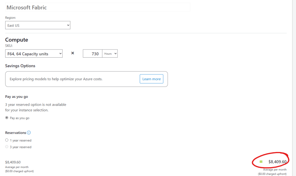
To get an overview and give you a better idea of what is the best option for you, the Azure Pricing Calculator can be used. You type Fabric in the search box and choose the Microsoft Fabric option as shown below.
A screenshot of a computer

Description automatically generated

You then choose the Region, Compute Sku (capacity) and pricing model. For example, choosing a F64 capacity for 730 hours (1 month) costs USD $8409.60 with no upfront costs.

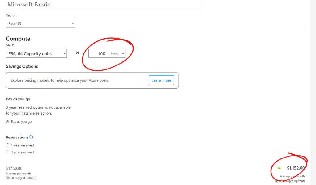
If we choose the Pay-as-you-go model, we want to Pause and resume the capacity upon our usage. The same F64 capacity cost would be reduced to USD $1152.00 if we use it only 100 hours per month (12 days approx.)

But if we use the 1-year reserved plan, the price reduction is quite interesting: USD $5002.67.

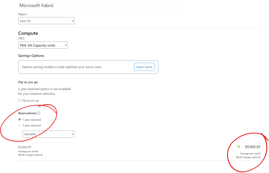
We can choose the 1-year reserved option for lower capacity as well. Prices differ by region, so ensure you select the correct region before estimating costs.

Conclusion

Both the Pay-as-you-go model and the Reserved 1-year plan offer distinct advantages for obtaining copilot capacities with Fabric

As you consider these options, keep in mind that the goal is to leverage copilot capacities to their fullest potential, driving innovation and achieving excellence in your business operations. Whether you opt for the flexibility of Pay-as-you-go or the savings of a Reserved 1-year plan, the key is to remain adaptable and responsive to the ever-evolving demands of the digital age.
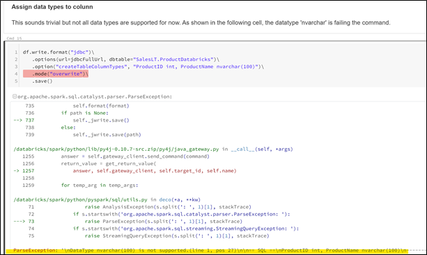
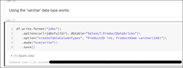
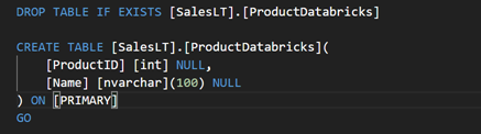
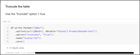
Unleashing the Power of Fabric Data Warehouse Copilot


Unleashing the Power of Fabric Data Warehouse Copilot

Microsoft Fabric has introduced a groundbreaking AI assistant designed to revolutionize your data warehousing tasks: Fabric Data Warehouse Copilot. This innovative tool integrates seamlessly with your Fabric warehouse, providing intelligent insights and streamlining operations to enhance productivity.

This article is the first of a series of articles on the topic of Copilot integration with Microsoft Fabric.

Introduction to Fabric Data Warehouse Copilot

Fabric Data Warehouse Copilot is an AI assistant specifically designed to assist with data warehousing tasks. It leverages the power of generative AI to give intelligent insights, automate key aspects of data management, and enhance the overall efficiency of SQL developers and analysts.

Key Features of Fabric Data Warehouse Copilot

  1. Natural Language to SQL: One of the standout features of Copilot is its ability to generate SQL queries using simple natural language questions. This feature allows users to interact with their data warehouse in a more intuitive and user-friendly manner.
  2. Code Completion: Copilot enhances coding efficiency by providing real-time, context-aware code completions directly in the SQL query editor. This feature helps reduce errors and speeds up the development process.
  3. Quick Actions: Copilot offers quick actions such as “Fix” and “Explain” for SQL queries. These actions allow users to quickly address errors and understand their queries better, making the development process smoother and more efficient.
  4. Intelligent Insights: Copilot provides smart suggestions and insights based on the warehouse schema and metadata. This feature helps users make informed decisions and optimize their data management processes.
  5. Chat Pane: Users can ask questions to Copilot through the chat pane using natural language. Copilot responds with generated SQL queries or natural language explanations based on the questions asked.

This article will focus on the natural language to SQL mainly and the code completion features.

Prerequisites

Here is a short list of what is needed to use copilot with a data warehouse in Fabric:

The data model

I created a data warehouse for this article series to show how code completion can help with all the functionalities. I designed in a star schema format, originating from the AdventureworksLT database. Here is the model:

Very important: I defined all the foreign key relations as they help Copilot to better understand the data model and returns better results.

Natural language to SQL

This data model looks nice, but it is missing role-playing dimensions for the various date columns in the FactOrders table:

  • IDDueDate, we’ll create a view on top of the DimDate dimension called DimDueDate
  • IDOrderDate, we’ll create a view on top of the DimDate dimension called DimOrderDate
  • IDShipDate, we’ll create a view on top of the DimDate dimension called DimOrderDate

To create those views, I opened a new SQL query window in Fabric and types the next command:

Copilot generated a preview (in gray) and I saw what SQL statement should be issued. I didn’t like the “SELECT *” in the SQL statement. So I was more precise in my second try and asked Copilot to avoid using the “SELECT *” in the code to be generated:

The generated SQL looked better but I didn’t like the format of the code, every column on a single line. I tried to be more specific again and my 3rd try was quite successful:

I am not a big fan of using the dbo schema in SQL. So, I asked Copilot to create a schema called “Enriched”:

For fun, I tried to be even more precise, I told Copilot to alias the DimDate table and rename the IDDAte column:

I accepted the result this time. I repeated the same process for the two other view. Here’s a screenshot of the final model.

If you are new to a data model like that one (even if it’s simple), Copilot can be used to describe the data model. I opened another SQL query pane, and I typed the next command:


— create a description for all the database objects

Using the Code Completion feature

As mentioned in the above section, I am not a big fan of the dbo schema. But all my tables were created in it. So, I decided to use code completion to make me more productive in that area. The syntax to move table from dbo to my Enriched schema is the following:
ALTER SCHEMA Enriched TRANSFER dbo.<my table>;

In a query pane, I started typing the command for the first table that I wanted to transfer. It didn’t work as intended at first. But Copilot learned what I wanted to do after a few attempts, and I got the following help from it:

I accepted and cleaned up the code as not every tables/views needed to be transferred. But again, Copilot was a great helper here.

I then tried to create a stored procedure that return the result of all my tables joined:

Interestingly, a query was created instead of a stored procedure 😊. The result is not perfect but good enough to get me started with a stored procedure creation.

Maximizing Productivity with Copilot

The few examples of this article demonstrated how Copilot can make the next personas more productive:

  • The data analyst
    • Understand and document the database content
    • Create queries using natural language
  • The data architect to create database objects, move and rename database objects
  • The TSQL developer can use it to create queries and use them in stored procedures or functions.

Conclusion

Fabric Data Warehouse Copilot, while still in public preview, will become a powerful AI assistant that can transform the way we manage our data warehouse. By leveraging its natural language to SQL capabilities, code completions, we can streamline our data warehousing tasks and boost productivity.

Whether you’re a seasoned SQL developer or a business analyst, Copilot is here to help you unlock the full potential of your data warehouse. I will write a few other articles on Copilot with Fabric Data Warehouse to fully experiment and explain the various features. I will certainly come back to the code completion and show more of it from a TSQL developer perspective as the product evolve and gets better.

Give a mixed case name to your Delta table

Whenever we create a Delta table using the write(). format(‘delta’).saveAsTable(‘DimCustomer), the table will be named “dimcustomer”. The table’s columns can use mixed case, but it seems that saving a table using mixed case – DimCustomer with capital D and capital C cannot be done with Spark default options. If we use Fabric Data Factory, we can specify DimCustomer in the target table and the table name will not be lowercased.


And the resulting table will be named with mixed-case.


But when we use a notebook (code) to create the table, things are a bit different as shown below. The table name is dimcustomer, no upper-case letters, no mixed case letters.


This is a bit annoying to me. I looked on the web and I couldn’t find a way to name a Delta table with mixed or uppercase. The I found an article that talked about case sensitivity with Spark by using a config command : spark.conf.set(‘spark.sql.caseSensitive’, False).

I used it in my code and voilà! I now have a table name with mixed case! The only thing I had to do was to drop the table before. I could not use the “overwrite” option to simply rename the table. But I don’t have to do it in my subsequent loads.


Hope this article will help people that had the same issue I had with Delta table names!

Do we need database in a Data Analytic project

With the growing popularity and use of data lakes and big data services in the cloud, people are questioning the need of a database in their analytic solution. This article will talk about how a database fit in a modern analytic architecture.

The data Lakehouse

Data lakehouses are being more and more used in the industry. They combine every resource needed to ingest, clean, transform and present data to consumers. These consumers can be other systems like machine learning workspaces and other API’s as well as data science notebooks and BI report users. They can ingest and store all kinds of data as described in the following table.

Type of data

Description

Examples

Unstructured

Data without any usable structure

Text documents like PDF files, word processing and image files. Media filles like music or videos.

Semi-structured

Data have some structured element but without formal or strict organization of them.

Log files from IoT systems, Json and XML, web pages, etc.

Structured

Data is organized into a formal schema.

Database, Excel spreadsheets, delimited files, etc.


Major vendors support data lakehouse features such as Databricks, and Microsoft Synapse Analytics. Databricks introduced the Delta Lake project and open sourced it in early 2019. It brings the following benefits to a data lake:

  • Delta Sharing: enable data sharing from Delta tables with other systems without having to copy it before.
  • ACID transactions: Ensure data integrity.
  • Time travel: data is snapshotted, and every change made to it can be viewed and used by your pipelines. It helps when we need to revert a specific version of the data or audit it.
  • Parquet file format, an open-source format, is leveraged for its compression and encoding schemes.
  • Delta tables can be filles using both streaming and batch processing.
  • Schema is enforced to prevent bad data and help enforcing data quality.
  • Schema evolution: although not recommended in a production environment, this feature allows to change the schema over time. A simple option (mergeSchema) allows to add new columns to a table. For a productionized environment, proper DDL statements like ALTER TABLE are more suitable to prevent pipeline failures down the road.
  • Update, Merge and Delete support: Prio to Delta, data was loaded in append only mode. DML statement can now be used with Delta tables.

A complete exhaustive list of Delta tables features can be found on Delta.io web page. Delta tables can be integrated into Azure Synapse Analytics quite easily as it is supported by both SQL Serverless and Spark pools. Data factory and Synapse pipelines have direct connectors for Delta tables.

Microsoft is developing a similar concept in Synapse Analytics called Lake Database. These databases can contain tables that are linked to an Azure Storage account folder or file. They are still in preview as the time of writing, and they support CSV and Parquet file format. What’s nice with the Lake Database tables is that we have a designer inside Synapse Analytics to design our tables based on our files. Microsoft also offers templates that are out of the box solutions for a database such as Accounting, Customer, etc. Like Databricks Delta, Lake Database tables can also be used by SQL Serverless Pools, Spark Pools as well as Data factory and Synapse pipelines Since the Lake databases are quite new, I will write other articles on that topic in the coming weeks.

The role of the database in the mix

So, if we’re using Delta tables or Lake Database tables, can we query them directly using various methods like Azure Synapse workspaces, Power BY, etc. Do we still need a database? The answer is most of the time, yes. As good and powerful data lakes are, they are still struggling to deliver fast query results. Databricks added a new query engine called Photon a few months ago, but it might become quite expensive with heavy usage. It requires computation services to be up and running all the time to serve the analytic report needs. Data lake databases do not have features like granular row and column level security, dynamic data masking to hide certain fields values, etc.

Also, someone will want to compare or integrate the data lake tables with their existing application or database systems. Although Synapse Analytics provides access to the data lake files, other systems mighty not have this capability out of the box. Some data mart patterns like SCD Type 2 are better handled in a database as opposed to a data lake implementation.

Flexible and scalable

But the main reason to keep the database into an Analytical solution IMHO is flexibility and scalability. Flexibility, I can use multiple databases on top of my data lake for specific purposes or different business processes. I can use an Azure Serverless SQL database for small workloads and save money by not having a compute engine, read cluster, running all the time. I also have the possibility to scale up and down my database depending on my end user’s needs. I can even stop the database engine outside business hours the same way I could stop my data lake compute engine.

Helping report users

Another factor where having databases in our solution can help is that, while the data lake contains tons of data, my systems might only need a subset of it. For example, most of my reports might be using current or short-term data most of the time to render as fast as possible. I saw end users waiting for minutes for some reports that spawned over only a few months of data. The problem was that the database model was not optimized for such reports. People will easily understand that the report takes long time to render when we’re having many years of data to display. Such reports could easily be served by a specific connection to the data lake.

Performance optimizations

Databases have more handles in term of query optimizations compared to data lake tables. There are also more different database types when it comes to SQL Server in Azure. SMP databases like Azure SQL (serverless or managed instance, Hyperscale) or massive parallel processing (MPP) like Azure Synapse Dedicated pools can be used to expose data for different use cases. The former has replicated tables for dimensions and distributed tables for fact tables. Azure SQL database has also different types of indexes that can be used to optimize query performances.

Conclusion

The need for a database in an Analytical solution is still present even with modern data lake databases systems. The latter do not have all the features offered by good old relational databases. It’s better most of the time to segregate our workloads between the data lake for fast processing of big amount of data and using the database for mild transformation and consumption layer. This way, we get a secure, flexible solution that do not cost too much in term of operation and maintenance

SSIS vs TSQL and Azure migration perspectives

Microsoft always made SSIS flexible enough to enable developers to develop their ETL with different techniques. This article will talk about an old debate on how SSIS should be used as an ETL tool. I am sharing here my own experience on ETL’ing with SSIS and its implication when it comes to migrate our ETL’s to Azure.

The “DTS” way: using SSIS as an orchestrator

DTS (Data Transformation Services) has been around from the end of 20th century to the mid-2000’s. It relied on ActiveX technology to move and transform data. ActiveX was not very performant. ETL developers used DTS most of the time as an orchestrator of database stored procedures. Pipelines were designed to call a series of stored procedures that were doing data transformations. It was ELT, not ETL.

We can still use SSIS the same way we used DTS: use the control flow to orchestrate stored procedures. But there are a few caveats with this approach:

  • SSIS is not used to its to its full potential. Stored procedures still run on the database server and might create contention of resources on it.
  • Harder to tune-up performances: from an SSIS perspective, a stored procedure is a black box. SSIS has no clue on what’s going on when it runs a stored procedure, it simply calls it. I’ve seen stored procedures called in a dataflow OLE DB some executing very poorly. These dataflows were very hard to debug when they jammed, performances were slowing down or maintain because majority of transformations (if not all) were done in the underlying stored procedure.
  • Transformations logic are hidden: a dataflow task in SSIS exposes the transformations and it’s easy to understand the transformation flow.
  • Database might require supplemental indexes or views to speed up or ease the ETL process.

Bottom line, if you use TSQL to do the ETL, using SSIS is a bit overkill as the tool can do the same kind of transformations and many more.

Using the SSIS Data Flow

The SSIS data flow task has a lot of transforms available in its toolbox. They can read data and write from a variety of data sources like databases, files, on-premises Hadoop files, etc. With the addition of Azure Feature Pack, data can be read/written in various format like Avro or Parquet to an Azure storage. Data flows have a rich set of optimized transformations that allow doing all kind of transformations like pivoting or unpivoting the data, adding or modifying columns in the pipeline or simply joining or splitting data.

Data Flows are transforming the data in memory, so the performance greatly improved. They use strong data types that helps optimize memory consumption throughout the various transformations’ usage. Between every transformation, we can view the transformed data by enabling data viewers. They help greatly to develop or debug a transformation. Using various transformations leads to changing the way we design our ETL’s: we spread out and expose our transformation logic on the Data Flow design pane. Doing it allows to make our package more self-documenting and much easier to maintain.

There is also a quite large commercial third party’s components that provides lots of useful extension to SSIS. IF you ever need to read or validate a JSON file, read and write to a SharePoint list, there are components available for all of these.

Bottom line, if you’re using SSIS, the Data Flow task is your friend when it comes to data transformations. Of course, you can still use TSQL when it makes more sense. Let’s say you have two OLE DB sources in your package: Source A brings 1 million rows and Source B 1000. Both sources ar pulling data from the same RDBMS and inner joining the two sources would result to a dataset of 50000 records. It make sense to join the two sources in a single OLE DB source. Otherwise, bringing 1 million rows to the pipeline and filtering down 950 000 would make SSIS doing the join much slower that using the database for the same job.

Cloud migration perspectives

Migrating SSIS vs TSQL stored procedure to the cloud, Azure, can be easily done using the two following techniques:

  1. Lift and Shift of the ETL programs in Azure and use them almost as is.
  2. Re-write the ETL programs and ensuring the migration embrace the full cloud scalability paradigm.

If you’re using TSQL, you have to male sure that the Azure database supports all code syntax you used when it was developed on an on-premises server. If you’re using SSIS, you will need Azure Data Factory with its SSIS Integration Runtime to run your packages in Azure almost as is.

Doing a simple lift and shift does not mean that we’re using the Azure cloud technologies at its full potential. A re-write is required for that. This can be done by three major ETL technologies in Azure:

  • Azure Data Factory: using the mapping data flows of this technology, we can specify the joins and partitioning strategy that help distribute the ETL to many workers.
  • Azure Synapse: Microsoft is extending what was known as Azure Data Warehouse to create a unified Analytics experience. This technology will leverage parallel ETL distribution as it always did but this time, Spark is added to the mix.
  • Azure Databricks: This is a Spark specific technology, so it means that distributed processing is a no brainer for this one.

Now, if we use TSQL and want to migrate our ETL’s, we will have to reverse engineer our TSQL code and re-write the logic using one of the technologies stated above to ensure we’re fully using cloud at its full potential. If we’re using SSIS with the data flow, all the logic should be displayed in the package making the re-write much easier, especially if Data Factory and mapping data flows are leveraged. Data Factory data flows use many transformations found in SSIS data flows, so ETL logic migration should be very easy to do.

If Databricks is used, many TSQL can run leveraging SQL but since it’s not TSQL, some modifications to the code might be necessary as not all TSQL syntax is supported in Databricks. With SSIS, it means a complete re-write of the ETL. But since the logic is spread out in the data flows, it should be easy to migrate the sources and do transformations using DataFrames.

Bottom line, cloud migration is not a simple flip of the switch. Some work as to be done. Microsoft has a tool for that can greatly help us to asses the complexity for a Lift and Shift of our code: Data Migration Assistant. For a re-write, there’s no tool for it . I whish there was a tool that would script our SSIS packages to PySpark dataframe though. That would certainly be very helpful for lots a people.

Avoid SQL Server nvarchar(max) data type mapping in Databricks

When using dataframes and save it to SQL Server using JDBC, the resulting data type for a string column is nvarchar(max). This happens when let JDBC creating the table without supplemental instructions. We seldom need to have our string columns using with this data type as it limits the functions we can use with it such as substring().

This article will show some options to avoid having a nvarchar(max) column in our table

A simple query

First thing first, we’ll connect to a database. For this article. I am using a sample database; AdventureworksLT from Microsoft Git web site. With Databricks, we connect to the server using JDBC and query the “SalesLT.Product” table to bring back two columns:

  • ProductID: integer column;
  • Name: navarchar column, it will be seen as a string in the dataframe;

Now that we have retrieved data in our dataframe, we’re going to save it back in a different table. In real life, we would have transformed the data quite a bit but yhe goal of this article is to explain how to save a dataframe back to SQL Server with correct data types.

Save the dataframe; the simple way

The first thing we will do is to simply save, overwriting the destination table. Overwriting the table without any other options means we are going to drop and recreate the table.

The resulting table structure is shown below. I did the screenshot with Azure Data Studio. As we can see, the “ProductName” column’s data type is nvarchar(max). This is not the best option but, it ensures that whatever is stored in the dataframe’s string column will fit; it’s a safe choice.

There’s a way to specify the data type of the dataframe’s columns while saving it to the database. But in order to find the right length, we need to profile the data. Still in Databricks, we’ll find the maximum length of the “ProductName” column in our dataframe as shown below.

Specifying a data type

Now that we know the maximum value in the column, we use the “createTableColumnTypes” option when we save the dataset. However, specifying “nvarchar(100)” fails. The “nvarchar” data type is not supported for now.

Using the “varchar” data type executes successfully as shown below.

When we look at the table structure in Azure Data Studio, we clearly see that the command created a table with the specified structure.


However, I am not satisfied with it. I dislike using “varchar” data type as we live in a connected world now and sooner or later, this data type will limit us with international character sets. To circumvent this, we have to create the table first as shown below.

Truncate the table

Next, we’ll use the “truncate” option with the save command. This will NOT drop and recreate the table but simply empty (truncate) the table.

Going back to Azure Data Studio, we notice that the table’s structure has not been altered by the save with overwrite command.


But we have to be careful because if the structure of the dataframe changes by adding/renaming a column, the command will fails as shown below.


To sum up

There are some valid options to avoid be stucked with a “nvarchar(max)” column while saving a dataframe with Databricks An improvement I would like to see is the support for “nvarchar” data types. This might come in a near future.

SSIS Error: Cannot process request in SSDT

I was recently deploying a SSIS project to another server recently and I encountered the following error:

Microsoft Visual Studio

——————————

Cannot process request because the process (114328) has exited.

I searched on the web to find out what could be causing this error. Project opened on my development machine executed flawlessly. Of course, we cannot use my development machine as an execution server , so I had to find the answer.

When we create a SSIS project in SSDT/Visual Studio 2017, the deployment target server is set to SQL Server 2017. I hadn’t change it when I created the project and was tryin to execute a package on SSIS 2016…this was my mistake.


I simply set the Deployment Target Server (right-click on the SSIS project à Configuration Properties) of my dev machine SSIS project to SQL Server 2016 and the issue was gone!

Simple things like that sometimes make us loose lots of valuable time! Hopefully this article will help some of you as the error message I got was not really helpful.


Databricks-cli setup

Databricks-cli is used for the Databricks administration. With it, we can manage the following items:

  • Clusters:     Utility to interact with Databricks clusters.
  • Configure:     Configures host and authentication info for the CLI.
  • Fs:         Utility to interact with DBFS.
  • Groups:        Utility to interact with Databricks groups.
  • Jobs:        Utility to interact with jobs.
  • Libraries:    Utility to interact with libraries.
  • Runs:         Utility to interact with the jobs runs.
  • Secrets:     Utility to interact with Databricks secret API.
  • Stack:        Utility to deploy and download Databricks resource stacks.
  • Workspace :     Utility to interact with the Databricks workspace.

The remainder of this page will describe how to setup Databricks-cli.

Requirements

We need an access to a Databricks workspace’s token. Also, Python has to be installed on the developer’s PC.

Python installation

From https://www.python.org/downloads/windows/, download the latest Windows version as shown in the following screenshot. You can opt for the web or full installer, One or the other doesn’t matter.

Once the setup starts, you’ll get the following screen (the Python version may differ).

Make sure that the two checkboxes are selected :

  • Install launcher for all users
  • Add Python to PATH

Once the installation completes, go to the environment variables of your PC:

Click on environment variables

Select Path in the “User variables” (upper window) and  click on “Edit” as highlighted below.

Click on New as shown below

Enter the following string:

%USERPROFILE%\AppData\Local\Programs\Python\Python37\Scripts

And click on OK in both windows to save the path as shown below.

Open a command window and type the following command:

pip3 install databricks-cli

The installation will go on. At the end of it. Open to the %USERPROFILE%\AppData\Local\Programs\Python\Python37\Scripts folder and you should see  “Databricks.exe” as shown in the following screenshot.

Now, back to the command window, type the following command:

databricks --version 

The version of databricks should now be displayed as shown below.

We’re now ready to configure databricks-cli.

Databricks-cli configuration

Once databricks-cli is installed, we have to connect to an existing Databricks workspace. In order to do so, we’ll use the following command:

databricks configure --token

as shown in the following screenshot.

The Databricks host is where  Azure region where the workspace has been created; in our case, East US. The token can be obtained from the workspace itself. Here’s the procedure to do it. Open the Databricks workspace you want to link to the databricks-cli and follow this link to create the token for the workspace.

Databricks Load XML libraries

AT my client’s place we’re using Databricks in conjunction with Azure Data Factory to transform data coming from HTTP connections. These connections data end up in an Azure blob. When we’re receiving JSON data, Databricks and most Azure components knows how to deal such data. Databricks have JSON libraries already available for us to use.

We start receiving XML files from a provider lately. Using Databricks, I thought that I would be able to load the data in a data frame as easily than I am doing with JSON from the Azure blob storage. Here’s the command I use in Python to load JSON data:

df = spark.read.option(“multiLine”, True). json(completeFilePath)

The command tells Databricks to load my “completeFilePath” content from my blob storage into a data frame called “df”. I use the “multiline” option because the JSON data is spanning on multiple lines.

Naively, I thought that reading an XML file would be as easy. I just have to issue a command like the following in Python:

df = spark.read.option(“multiLine”, True). xml(completeXMLFilePath)

Unfortunately, this is not that easy. There’s no native XML library available with Databricks when we create a workspace. We need to load one. After some research on the web, I found this link on Github: https://github.com/databricks/spark-xml. In the document, we can download the library and we need to load it in the notebook. Here are this instructions on how to refer to the libfrary in the notebook.

Spark compiled with Scala 2.11
$SPARK_HOME/bin/spark-shell –packages com.databricks:spark-xml_2.11:0.4.1

From a Databricks notebook perspective, this is not obvious how to attach the library to it. We cannot use this code anywhere in the notebook. I don’t pretend to be a Databricks expert though but even when I looked at the cluster configuration, I could not find a way to attach such library as shown in the following screenshot

Even not from the Libraries tab:

Doing more research on the web pointed me to the right place. From the notebook folder menu, we click on the drop down arrow, select Create and then Library from the submenu that appears as shown below.

The following screen appears. Select Maven Coordinate as source and click on the “Serach Spark Packages and Maven Central button after.

From the search page, type “xml” and click on the search magnifier icon as shown below. From the list that appears in the center, select “spark-xml”, choose the release that matches your cluster, 2.11 in my case and click on “+ Select” right beside it as shown below.

The screen close and you’re back to the “Create Library” screen. Click on the “Create Library” button at the bottom of the screen.

The next screen allows us to attach the library to a cluster. Click on the “Attach automatically to all clusters.” If you want to be able to use it with any cluster you create whether it’s a job or interactive cluster. Since we’re calling our notebook from Azure Data Factory, it’ll be a job cluster. This checkbox has to be checked for us.

When we select the checkbox, we get a confirmation window, click on “Confirm”. You should see that the library is attached once done.

Going back to the Cluster’s library tab, we now see that the library is attached to it.

Voilà! The library is attached and ready to use. From our notebook, we can now load a file any issuing the following command:

df = sqlContext.read.format(‘xml’).options(rootTag=”‘<my root tag>”).load(completeXMLFilePath)

And the dataframe “df” gets loaded with the “completeXMLFilePath” file content from our blob storage.

Hope this article will save you some time as I spend a couple of hours to find out how to attach the XML library to my clusters.

Usefull Visio templates

A great part of my work has to do with documentation and diagramming. I'm always using various templates and I'll share them in this blog article.

Hope this helps you when you have to document your architecture!

Blog at WordPress.com.

Up ↑